Creating an AI that picks your best photo
Introduction
You’ve probably experienced this: You want to upload a photo to social media, so you open your gallery, only to find 300 almost identical pictures to choose from. Wouldn’t it be nice to have an AI highlight the best ones, so you don’t waste time scrolling through all of them? Let’s try to build that AI.
General idea
First we need to define what “best” means here. It needs to be something quantifiable. Let’s consider the photo that would get the most likes as the “best”. To normalize this, we’ll look at the ratio of likes relative to the average number of likes a user receives. From now on we’ll call this the “likes ratio”.
$$\text{{likes ratio}} = \frac{{\text{{likes}}}}{{\text{{average likes}}}}$$We’ll consider this as a regression problem. The inputs to the model will be the image plus some metadata, and the output will be the predicted likes ratio. This will be the “score” that each photo is assigned, so we’ll sort by this score to show the best pictures. I tried using other metrics for the output score, such as the predicted number of likes (instead of the likes ratio), but this approach worked somewhat better.
The metadata I mentioned includes features such as the average number of likes that a user receives, follower and following counts, the age of the photo, and so forth. During training, we input the correct values. During inference, we input generic values for the metadata, with the image being the only actual input. In principle, however, the model could learn about different cohorts based on attributes such as followers and followings (influencers, brands, regular people, etc.), so using simulated metadata in line with the characteristics of the user querying the model could better tailor the image assessment for them.
Dataset
| Number | Mean | Std | Median | Min | Max | |
|---|---|---|---|---|---|---|
| Profiles | 12101 | |||||
| Posts | 133418 | |||||
| Post Likes | 27640 | 287716 | 229 | 1 | 25094192 | |
| Profile Avg Likes | 27640 | 253955 | 261 | 20 | 9694053 | |
| Followers | 975543 | 10061096 | 9243 | 82 | 455547558 | |
| Following | 1347 | 1344 | 989 | 0 | 8293 |
The dataset consists of ~202k images before filtering, and ~133k images after filtering, each annotated with the number of likes, the average number of likes that the user receives, follower/following count, the date of the post, and the date when the data was obtained. As we’ll discuss later, although I achieved decent results using this dataset, the dataset is too small for optimal results.
The data was filtered using the following criteria (only the posts that met all these criteria were included):
Average likes >= 20: To exclude very noise samples
Post count >= 6: To exclude users with too few posts
Max Likes / Min Likes <= 25: To exclude users with very a high variance of likes, which was usually related to fishy accounts (bought likes, bots, etc).
Post age > 24 Hours: To exclude posts that are too recent and the number of likes is still far from reaching a stable value. The number of likes of course will still be correlated to the post age, but hopefully the model will learn this correlation (as age is one of its inputs) and correct for it.
Originally I tested on an even smaller dataset, and every time I increased the dataset size, the accuracy would significantly increase.
We’ll be using a 80/20 train/validation split.
Inputs and outputs
We’ll use the following inputs:
- Image 224x224 RGB
- Log(Average Likes): Logarithm of the average number of likes for the user
- Log(Days ago): Logarithm of how many days old the post is
- Cyclical Encoding(Day of the week): Cyclical encoding (sin and cos) of the day of the week [0, 6]
- Cyclical Encoding(Time of day): Cyclical encoding (sin and cos) of the minute of the day [0, 1439]
- Log(Followers): Logarithm of follower count
- Log(Following): Logarithm of following count
The output will be:
- Log(Likes/Average likes): Logarithm of the likes ratio of this post
Given how large the variance of most of these inputs are, they are normalized using the natural logarithm. The day of the week and time of day are encoded using cyclical encoding, due to the cyclical nature of these values. This means that each is converted into two scalars (sine and cosine). The output also has Log applied, as it seemed to work better than simply using Likes/Average Likes, or even Likes/Average Likes - 1 (to normalize it to a mean of 0).
The dataset code looks something like this:
class CustomDataset(Dataset):
    def __init__(self, posts, transform=None):
        self.posts = posts
        self.transform = transform

    def __len__(self):
        return len(self.posts)

    def __getitem__(self, idx):
        def cyclical_encoding_day(dt):
            # Extract the day of the week as an integer (0: Monday, 1: Tuesday, ..., 6: Sunday)
            day_of_week = dt.weekday()

            # Perform cyclical encoding using sine and cosine functions
            day_sin = math.sin(2 * math.pi * day_of_week / 7)
            day_cos = math.cos(2 * math.pi * day_of_week / 7)

            return day_sin, day_cos

        def cyclical_encoding_time(dt):
            # Extract the hour and minute
            hour = dt.hour
            minute = dt.minute

            # Compute the minute of the day
            minute_of_day = hour * 60 + minute

            # Perform cyclical encoding using sine and cosine functions
            time_sin = math.sin(2 * math.pi * minute_of_day / (24 * 60))
            time_cos = math.cos(2 * math.pi * minute_of_day / (24 * 60))

            return time_sin, time_cos

        post = self.posts[idx]

        # Use the already cropped image
        image_path = post['image_path']
        image_path = image_path.replace('images/', 'images_cropped/')

        # Use log to normalize the data
        log_likes_ratio = np.log(post['likes'] / post["avg_likes"])
        log_avg_likes = np.log(post["avg_likes"])
        log_followers = np.log(post["followers"] + 1)
        log_following = np.log(post["following"] + 1)

        post_time = post["post_time"]
        scrap_time = post["scrap_time"]
        log_days_ago = np.log((scrap_time - post_time) / (24.0 * 60.0 * 60.0) + 1)

        # Normalize
        log_followers /= 15.0
        log_following /= 15.0
        log_days_ago /= 10.0

        # Encode the day of the week and time of the day using cyclical encoding
        post_time_dt = datetime.datetime.fromtimestamp(post_time, tz=datetime.timezone.utc)
        post_time_day_sin, post_time_day_cos = cyclical_encoding_day(post_time_dt)
        post_time_time_sin, post_time_time_cos = cyclical_encoding_time(post_time_dt)

        label = torch.tensor([log_likes_ratio], dtype=torch.float32)
        metadata = torch.tensor([log_avg_likes, log_days_ago, post_time_day_sin, post_time_day_cos, post_time_time_sin, post_time_time_cos, log_followers, log_following], dtype=torch.float32)

        img = Image.open(image_path)

        if self.transform:
            img = self.transform(img)

        return post["post_id"], img, metadata, label
Note that we include the post_id because it will be useful later on for calculating accuracy.
Model
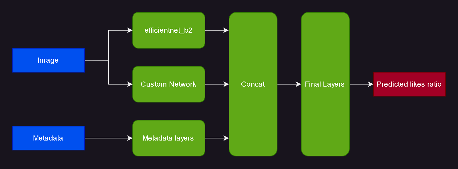
I spent quite some time trying various architectures until I arrived at the one shown in the figure. There were a few constraints
- It should avoid overfitting the very small dataset
- It should take into account certain information that is usually thrown away for your typical classification problem
- It should train relatively quickly, so I could iterate a lot
For the image processing part, it uses a pretrained model from timm, plus a custom model. For the metadata, it uses a couple fully connected layers. Then everything is concatenated, passed through a couple more fully connected layers, and finally you get your output.
efficientnet_b2: This is a pretrained model from EfficientNet: Rethinking Model Scaling for Convolutional Neural Networks. Specifically, tf_efficientnet_b2.ns_jft_in1 is used, which has been pretrained on JFT-300M—an internal Google dataset—and subsequently on the ImageNet-1K dataset. During training, the first few layers of the model are frozen to mitigate overfitting. In addition, a fairly high dropout of 0.7 is used throughout the model to further combat overfitting.
Custom Network Your typical image classification model is designed and trained to overlook elements such as variations in image brightness, contrast, and general color grading. In this specific case, however, these features are of great importance. Therefore, a custom network is incorporated with the hope of capturing these attributes. It consists of a substantial downsampling step that results in a 3x14x14 image, followed by three fully connected layers. The implementation of this network appears to increase accuracy by a few percentage points.
Metadata Layers: Two fully connected layers so the metadata can be processed a bit before being concatenated with the visual features.
Final Layers: Two fully connected layers followed by a final linear layer to calculate the final output.
The final model ends up looking like this:
class ColorGradingFramingNet(nn.Module):
    def __init__(self):
        super().__init__()

        self.downsample = nn.AvgPool2d(kernel_size=16, stride=16)
        self.features = nn.Sequential(
            nn.Linear(14 * 14 * 3, 32),
            nn.SiLU(),
            nn.Linear(32, 32),
            nn.SiLU(),
            nn.Linear(32, 16),
            nn.SiLU(),
        )

    def forward(self, x):
        x = self.downsample(x)
        x = torch.flatten(x, 1)
        x = self.features(x)
        return x

class CustomNetwork(nn.Module):
    def __init__(self, num_metadata=8):
        super().__init__()

        self.model1 = timm.create_model("tf_efficientnet_b2.ns_jft_in1k", num_classes=0, pretrained=True, drop_rate=0.7, drop_path_rate=0.7)
        self.model2 = ColorGradingFramingNet()

        for param in self.model1.conv_stem.parameters():
            param.requires_grad = False

        for param in self.model1.bn1.parameters():
            param.requires_grad = False

        for layer_idx in range(4):
            for param in self.model1.blocks[layer_idx].parameters():
                param.requires_grad = False

        self.metadata_layers = nn.Sequential(
            nn.Linear(num_metadata, 32),
            nn.SiLU(),
            nn.Linear(32, 32),
            nn.SiLU()
        )

        self.final_layers = nn.Sequential(
            nn.Linear(1408 + 16 + 32, 128),
            nn.SiLU(),
            nn.Linear(128, 64),
            nn.SiLU(),
            nn.Linear(64, 1)
        )

    def forward(self, img, metadata):
        model1_features = self.model1(img)
        model2_features = self.model2(img)

        metadata_features = self.metadata_layers(metadata)

        x = torch.cat((model1_features, model2_features, metadata_features), dim=1)
        x = self.final_layers(x)

        return x
Data Augmentation
Data augmentation is a very powerful technique that allows your model to generalize better and prevent overfitting by creating modified copies of your images with different transformations, thus artificially increasing your training set. There are a wide variety of transformations available (see some examples here). For a typical image classification neural network, you would apply an extensive set of transforms, including drastically changing the colors of the image, cutting out parts of it, significant translations/rotations/crops, and more. Unfortunately, in this case we cannot do that, as we would be training the model to consider a heavily distorted with blown up colors photo to be as good as a properly framed photo with proper color grading.
So we’ll limit ourselves to transforms that only very lightly affect the image. Specifically, horizontal flips, 3 degrees rotations, 7.5% translations, and 10% scaling. Not being able to further augment the dataset makes overfitting a bigger challenge. Here’s the code:
# Very subtle transforms because we don't want to make the image uglier
# Normalize to imagenet
train_transform = transforms.Compose([
    transforms.RandomHorizontalFlip(),
    transforms.RandomAffine(degrees=(-3.0, 3.0), translate=(0.075, 0.075), scale=(0.9, 1.1)),
    transforms.ToTensor(),
    transforms.Normalize(mean=[0.485, 0.456, 0.406], std=[0.229, 0.224, 0.225]),
])

# Just normalize to imagenet for the validation set
val_transform = transforms.Compose([
    transforms.ToTensor(),
    transforms.Normalize(mean=[0.485, 0.456, 0.406], std=[0.229, 0.224, 0.225]),
])
Accuracy
It’s very beneficial to use a metric other than validation loss to assess the model’s performance. In this scenario, it’s a bit more complex than a typical classification problem.
We’ll group posts according to their users, and subsequently create pairs of posts. The model will then predict which post in each pair will receive more likes. We’ll gauge accuracy by the percentage of pairs correctly predicted by the model.
As for pair creation, if a user has five posts (ABCDE) after shuffling, we’ll form three pairs: AB, CD, and EA. This method allows us to test all the posts using the minimal number of pairs.
Training
Let’s start with the code and then explain some of the choices:
def main():
    # Load the dataset (posts)
    posts = get_posts()
    print(f"Loaded {len(posts)} posts")

    # Convert to a pandas dataframe
    df = pd.DataFrame(posts)

    # Get list of unique user_ids
    user_ids = df["user_id"].unique()

    # Split user_ids into 80% train and 20% validation sets
    split_idx = int(len(user_ids) * 0.8)
    train_ids = user_ids[:split_idx]
    val_ids = user_ids[split_idx:]

    # Filter the posts dataframes based on the user_ids from the splits
    train_df = df[df["user_id"].isin(train_ids)]
    val_df = df[df["user_id"].isin(val_ids)]

    # Convert the dataframes to lists of dicts
    train_posts = train_df.to_dict(orient="records")
    val_posts = val_df.to_dict(orient="records")

    # Group the validation df by user_id, to later create pairs of posts
    grouped_val = val_df.groupby("user_id")

    # Create pairs of posts beloinging to the same user.
    # If a certain user has posts A B C D E it will create
    # the pairs (AB) (CD) (EA)
    pairs = []
    for _, group_df in grouped_val:
        # Convert dataframe to a list of dicts
        group_posts = group_df.to_dict(orient="records")
        # Check if the user has more than 1 post (as you obviously can't create a pair otherwise)
        if len(group_posts) > 1:
            # Loop through the posts with an increment of 2
            for x in range(0, len(group_posts), 2):
                if x + 1 >= len(group_posts):
                    # Pair the last post with the first, if the is an odd number of post
                    pairs.append((group_posts[x], group_posts[0]))
                else:
                    # Pair the post with the following post
                    pairs.append((group_posts[x], group_posts[x + 1]))

    # Very subtle transforms because we don't want to make the image uglier
    # Normalize to imagenet
    train_transform = transforms.Compose([
        transforms.RandomHorizontalFlip(),
        transforms.RandomAffine(degrees=(-3.0, 3.0), translate=(0.075, 0.075), scale=(0.9, 1.1)),
        transforms.ToTensor(),
        transforms.Normalize(mean=[0.485, 0.456, 0.406], std=[0.229, 0.224, 0.225]),
    ])

    # Just normalize to imagenet for the validation set
    val_transform = transforms.Compose([
        transforms.ToTensor(),
        transforms.Normalize(mean=[0.485, 0.456, 0.406], std=[0.229, 0.224, 0.225]),
    ])

    # Hyperparameters
    batch_size = 256
    learning_rate = 0.001
    num_epochs = 10

    # Create the datasets with the respective transforms
    train_subset = CustomDataset(train_posts, transform=train_transform)
    val_subset = CustomDataset(val_posts, transform=val_transform)

    # Initialize the data loaders deterministically
    g = torch.Generator()
    g.manual_seed(0)
    train_dataloader = DataLoader(
        train_subset,
        batch_size=batch_size,
        shuffle=True,
        num_workers=4,
        persistent_workers=True,
        pin_memory=True,
        worker_init_fn=seed_worker,
        generator=g,
    )
    val_dataloader = DataLoader(
        val_subset,
        batch_size=batch_size,
        shuffle=False,
        num_workers=4,
        persistent_workers=True,
        pin_memory=True,
        worker_init_fn=seed_worker,
        generator=g,
    )

    # Use GPU if available
    device = torch.device("cuda:0" if torch.cuda.is_available() else "cpu")

    # Initialize model and send it to GPU if available
    model = CustomNetwork().to(device)

    # Use mean squared error loss
    criterion = nn.MSELoss()

    # Use AdamW
    optimizer = optim.AdamW(model.parameters(), lr=learning_rate, weight_decay=0.05)

    # Use the 1cycle learning rate policy from the Super-Convergence paper
    scheduler = torch.optim.lr_scheduler.OneCycleLR(
        optimizer,
        max_lr=learning_rate,
        steps_per_epoch=len(train_dataloader),
        epochs=num_epochs,
    )

    # Init AMP for mixed precision training to speed up training
    scaler = amp.GradScaler()

    best_val_loss = float("inf")

    # Training loop
    for epoch in range(num_epochs):
        # Record the start time of the epoch
        start_time = time.time()

        # Training
        train_loss = 0.0
        # Set model to training mode
        model.train()
        for post_ids, inputs, metadata, labels in train_dataloader:
            inputs, metadata, labels = (
                inputs.to(device),
                metadata.to(device),
                labels.to(device),
            )

            optimizer.zero_grad()

            # Use autocast to enable mixed precision
            with amp.autocast():
                outputs = model(inputs, metadata)
                loss = criterion(outputs, labels)

            # Scale the loss and perform backpropagation with the GradScaler
            scaler.scale(loss).backward()
            scaler.step(optimizer)
            scaler.update()

            train_loss += loss.item()
            # OneCycleLr steps every batch
            scheduler.step()

        # Validation
        val_loss = 0.0
        correct_predictions = 0

        # Set model to evaluation mode
        model.eval()

        # Dicts to cache outputs
        post_outputs = {}
        post_labels = {}

        # Disable gradient calculation to save memory
        with torch.no_grad():
            for post_ids, inputs, metadata, labels in val_dataloader:
                inputs, metadata, labels = (
                    inputs.to(device),
                    metadata.to(device),
                    labels.to(device),
                )

                # Use autocast for mixed precision during validation as well
                with amp.autocast():
                    outputs = model(inputs, metadata)
                    loss = criterion(outputs, labels)

                val_loss += loss.item()

                # Cache the label and output for every post id
                for i in range(len(post_ids)):
                    post_outputs[post_ids[i].item()] = outputs[i][0].item()
                    post_labels[post_ids[i].item()] = labels[i][0].item()

            # Calculate accuracy
            for (post1, post2) in pairs:
                # Get the outputs of labels from the cached values
                post1_output = post_outputs[post1["post_id"]]
                post2_output = post_outputs[post2["post_id"]]

                post1_label = post_labels[post1["post_id"]]
                post2_label = post_labels[post2["post_id"]]

                # If the predictions and labels agree on which image is better,
                # increase the number of correct predictions
                if (post1_output > post2_output) == (post1_label > post2_label):
                    correct_predictions += 1

        # Record the end time of the epoch
        end_time = time.time()

        # Calculate the elapsed time
        elapsed_time = end_time - start_time

        # Print epoch, train loss, validation loss, and time taken for the epoch
        print(
            f"Epoch {epoch+1}/{num_epochs} Train Loss: {train_loss/len(train_dataloader):.6f} Val Loss: {val_loss/len(val_dataloader):.6f} Accuracy: {correct_predictions / len(pairs):.4f} Time: {elapsed_time:.2f}s"
        )

        # If the validation loss is the best one yet, save the model
        if val_loss < best_val_loss:
            best_val_loss = val_loss
            torch.save(model.state_dict(), "model.pth")

    print("Finished Training")
    print(f"Best val loss {best_val_loss / len(val_dataloader):.6f}")
Dataset splits and validation pairs
    # Load the dataset (posts)
    posts = get_posts()
    print(f"Loaded {len(posts)} posts")

    # Convert to a pandas dataframe
    df = pd.DataFrame(posts)

    # Get list of unique user_ids
    user_ids = df["user_id"].unique()

    # Split user_ids into 80% train and 20% validation sets
    split_idx = int(len(user_ids) * 0.8)
    train_ids = user_ids[:split_idx]
    val_ids = user_ids[split_idx:]

    # Filter the posts dataframes based on the user_ids from the splits
    train_df = df[df["user_id"].isin(train_ids)]
    val_df = df[df["user_id"].isin(val_ids)]

    # Convert the dataframes to lists of dicts
    train_posts = train_df.to_dict(orient="records")
    val_posts = val_df.to_dict(orient="records")

    # Group the validation df by user_id, to later create pairs of posts
    grouped_val = val_df.groupby("user_id")

    # Create pairs of posts beloinging to the same user.
    # If a certain user has posts A B C D E it will create
    # the pairs (AB) (CD) (EA)
    pairs = []
    for _, group_df in grouped_val:
        # Convert dataframe to a list of dicts
        group_posts = group_df.to_dict(orient="records")
        # Check if the user has more than 1 post (as you obviously can't create a pair otherwise)
        if len(group_posts) > 1:
            # Loop through the posts with an increment of 2
            for x in range(0, len(group_posts), 2):
                if x + 1 >= len(group_posts):
                    # Pair the last post with the first, if the is an odd number of post
                    pairs.append((group_posts[x], group_posts[0]))
                else:
                    # Pair the post with the following post
                    pairs.append((group_posts[x], group_posts[x + 1]))
Splitting into the 80% training and 20% validation sets is a bit more complex here than your typical pytorch random_split. That’s because instead of just randomly dividing the posts, we divide the users into 80/20 groups, and then select the posts that belong to these users. Finally, we need the extra code to generate the pairs for accuracy calculation as described before.
Hyperparameters
    # Hyperparameters
    batch_size = 256
    learning_rate = 0.001
    num_epochs = 10
Set the hyperparameters. The batch size of 256 worked well on an RTX 3090, although it could probably be pushed to 512.
Datasets and Transforms
    # Very subtle transforms because we don't want to make the image uglier
    # Normalize to imagenet
    train_transform = transforms.Compose([
        transforms.RandomHorizontalFlip(),
        transforms.RandomAffine(degrees=(-3.0, 3.0), translate=(0.075, 0.075), scale=(0.9, 1.1)),
        transforms.ToTensor(),
        transforms.Normalize(mean=[0.485, 0.456, 0.406], std=[0.229, 0.224, 0.225]),
    ])

    # Just normalize to imagenet for the validation set
    val_transform = transforms.Compose([
        transforms.ToTensor(),
        transforms.Normalize(mean=[0.485, 0.456, 0.406], std=[0.229, 0.224, 0.225]),
    ])

    # Create the datasets with the respective transforms
    train_subset = CustomDataset(train_posts, transform=train_transform)
    val_subset = CustomDataset(val_posts, transform=val_transform)
Create the train and val datasets, each with their corresponding transform.
Data loaders
    # Initialize the data loaders deterministically
    g = torch.Generator()
    g.manual_seed(0)
    train_dataloader = DataLoader(
        train_subset,
        batch_size=batch_size,
        shuffle=True,
        num_workers=4,
        persistent_workers=True,
        pin_memory=True,
        worker_init_fn=seed_worker,
        generator=g,
    )
    val_dataloader = DataLoader(
        val_subset,
        batch_size=batch_size,
        shuffle=False,
        num_workers=4,
        persistent_workers=True,
        pin_memory=True,
        worker_init_fn=seed_worker,
        generator=g,
    )
It’s very important to initialize the Data Loaders with num_workers=4 (or higher) and pin_memory=True. Otherwise loading data will be a massive bottleneck during train time. worker_init_fn and generator are set to make the dataloaders deterministic.
Loss function
# Use mean squared error loss
criterion = nn.MSELoss()
Mean Squared Error is used. Other loss functions, such as Mean Absolute Error (MAE), did not perform as well. This is likely because the data has already been normalized with a logarithm, which consequently brings outliers closer.
Optimizer
# Use AdamW
optimizer = optim.AdamW(model.parameters(), lr=learning_rate, weight_decay=0.05)
AdamW is used. Weight decay is used to mitigate overfitting and make the model generalize better. I tried many times to use SGD, as it often generalizes better than Adam, and AdamW here was overfitting quite hard. However I never got SGD to beat AdamW with early stopping.
Scheduler
# Use the 1cycle learning rate policy from the Super-Convergence paper
scheduler = torch.optim.lr_scheduler.OneCycleLR(optimizer, max_lr=learning_rate*10, steps_per_epoch=len(train_dataloader), epochs=num_epochs)
I used the 1cycle learning rate policy from Super-Convergence: Very Fast Training of Neural Networks Using Large Learning Rates. In previous attempts Cosine Annealing also worked relatively well , but 1cycle proved superior.
Remember that you need to call scheduler.step() with every minibatch (instead of every epoch) when using 1cycle.
Mixed precision
I used Automatic Mixed Precision (torch.amp) to speedup training. It resulted in a ~2x training time speedup.
Training loop
    # Training loop
    for epoch in range(num_epochs):
        # Record the start time of the epoch
        start_time = time.time()

        # Training
        train_loss = 0.0
        # Set model to training mode
        model.train()
        for post_ids, inputs, metadata, labels in train_dataloader:
            inputs, metadata, labels = (
                inputs.to(device),
                metadata.to(device),
                labels.to(device),
            )

            optimizer.zero_grad()

            # Use autocast to enable mixed precision
            with amp.autocast():
                outputs = model(inputs, metadata)
                loss = criterion(outputs, labels)

            # Scale the loss and perform backpropagation with the GradScaler
            scaler.scale(loss).backward()
            scaler.step(optimizer)
            scaler.update()

            train_loss += loss.item()
            # OneCycleLr steps every batch
            scheduler.step()

        # Validation
        val_loss = 0.0
        correct_predictions = 0

        # Set model to evaluation mode
        model.eval()

        # Dicts to cache outputs
        post_outputs = {}
        post_labels = {}

        # Disable gradient calculation to save memory
        with torch.no_grad():
            for post_ids, inputs, metadata, labels in val_dataloader:
                inputs, metadata, labels = (
                    inputs.to(device),
                    metadata.to(device),
                    labels.to(device),
                )

                # Use autocast for mixed precision during validation as well
                with amp.autocast():
                    outputs = model(inputs, metadata)
                    loss = criterion(outputs, labels)

                val_loss += loss.item()

                # Cache the label and output for every post id
                for i in range(len(post_ids)):
                    post_outputs[post_ids[i].item()] = outputs[i][0].item()
                    post_labels[post_ids[i].item()] = labels[i][0].item()

            # Calculate accuracy
            for (post1, post2) in pairs:
                # Get the outputs of labels from the cached values
                post1_output = post_outputs[post1["post_id"]]
                post2_output = post_outputs[post2["post_id"]]

                post1_label = post_labels[post1["post_id"]]
                post2_label = post_labels[post2["post_id"]]

                # If the predictions and labels agree on which image is better,
                # increase the number of correct predictions
                if (post1_output > post2_output) == (post1_label > post2_label):
                    correct_predictions += 1

        # Record the end time of the epoch
        end_time = time.time()

        # Calculate the elapsed time
        elapsed_time = end_time - start_time

        # Print epoch, train loss, validation loss, and time taken for the epoch
        print(
            f"Epoch {epoch+1}/{num_epochs} Train Loss: {train_loss/len(train_dataloader):.6f} Val Loss: {val_loss/len(val_dataloader):.6f} Accuracy: {correct_predictions / len(pairs):.4f} Time: {elapsed_time:.2f}s"
        )

        # If the validation loss is the best one yet, save the model
        if val_loss < best_val_loss:
            best_val_loss = val_loss
            torch.save(model.state_dict(), "model.pth")

    print("Finished Training")
    print(f"Best val loss {best_val_loss / len(val_dataloader):.6f}")
A few things to note here:
Two dicts (
post_outputsandpost_labels) are used to cache the outputs and labels of the validation set when calculating the validation loss. This is so that later when we loop through the pairs for accuracy calculation, we don’t need to run the posts again through the model.The model is saved to disk only if it beats the previous best validation loss. This works as a form of early stopping, so that we save the model to disk before overfitting starts hurting the model performance.
Results
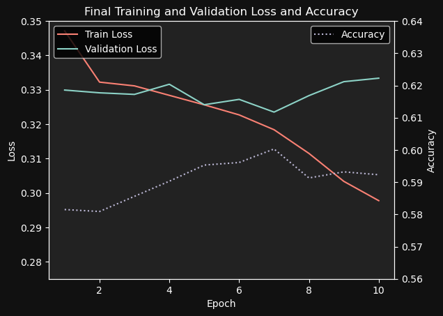
I trained the model for 10 epochs. Because of early stopping, the 7th epoch is the one that was actually saved to disk, as the model started to heavily overfit after that.
I tried training the model for more epochs with a lower training rate, but it didn’t perform as well.
Final results:
Training loss: 0.318381
Validation loss: 0.323505
Accuracy: 0.6003
A 60% accuracy was achieved. Clearly better than chance, but there’s room for improvement for sure. The most obvious way to improve the accuracy is to increase the dataset size. You’d probably want around 2M posts, but based on experiments I performed, any increase in the dataset size will yield very significant improvements to the accuracy. For example, increasing the number of posts from ~100k to the current ~133k increased the accuracy from 58% to 60%.
As we’ll see when testing the model, it is actually quite accurate when comparing two images where one is clearly inferior to the other. It’s when images are more comparable that it has trouble. Anecdotally, based on a very small sample size, my (human) accuracy on this dataset is around 70%.
Sampling
Now that the model is trained, let’s try to actually use it.
Let’s create a Jupyter Notebook and add the following code:
import torch
import torchvision.transforms as transforms
import matplotlib.pyplot as plt
from PIL import Image
import math
from models.model import CustomNetwork
from PIL import Image
import os


def resize_smallest_axis(img, target_size):
    width, height = img.size
    aspect_ratio = float(width) / float(height)
    if width < height:
        new_width = target_size
        new_height = int(target_size / aspect_ratio)
    else:
        new_width = int(target_size * aspect_ratio)
        new_height = target_size
    return img.resize((new_width, new_height), Image.Resampling.LANCZOS)


def center_crop(img, output_size):
    width, height = img.size
    new_width, new_height = output_size

    left = (width - new_width) / 2
    top = (height - new_height) / 2
    right = (width + new_width) / 2
    bottom = (height + new_height) / 2

    return img.crop((left, top, right, bottom))


def preprocess_image(path):
    resize_target_size = 224
    crop_output_size = (224, 224)
    img = Image.open(path).convert("RGB")
    img_resized = resize_smallest_axis(img, resize_target_size)
    img_cropped = center_crop(img_resized, crop_output_size)
    return img_cropped


def load_images():
    images = []
    for subdir, _, files in os.walk("test_images"):
        for filename in files:
            if filename.lower().endswith((".png", ".jpg", ".jpeg")):
                img_path = os.path.join(subdir, filename)
                images.append(preprocess_image(img_path))
    return images


def show_image(img, score):
    plt.style.use("dark_background")
    plt.figure(facecolor="#111")
    ax = plt.axes()
    ax.set_facecolor("#222")

    plt.imshow(img)
    plt.title(f"Score: {score:.3f}")
    plt.show()

# Use GPU if available
device = torch.device("cuda:0" if torch.cuda.is_available() else "cpu")
model = CustomNetwork().to(device)

# Load model
model.load_state_dict(torch.load('model.pth'))

# Set model to evaluation mode
model.eval()

# Load the images from the test directory
images = load_images()

# Use the following values for the simulated metadata
# Feel free to experiment with other values
avg_likes = math.log(250) / 15.0
days_ago_log = math.log(10) / 10.0
followers = math.log(10000) / 15.0
following = math.log(1000) / 15.0

val_transform = transforms.Compose([
    transforms.ToTensor(),
    transforms.Normalize(mean=[0.485, 0.456, 0.406], std=[0.229, 0.224, 0.225])
])

final_images = []
for img in images:
    input = val_transform(img).unsqueeze(0).to(device)
    metadata = torch.tensor([avg_likes, days_ago_log, 1.0, 0.0, 1.0, 0.0, followers, following], dtype=torch.float32).unsqueeze(0).to(device)

    # Get score from the models
    with torch.no_grad():
        score = model(input, metadata).item()

    # Normalize the score and modify it a bit so it's easier to interpret
    final_score = score
    final_images.append((img, final_score))

# Sort by score
final_images.sort(key=lambda x: x[1], reverse=True)

# Show the images with their score
for final_image in final_images:
    show_image(*final_image)
The code will iterate over all images in the test_images directory, center crop and resize them, run them through the model, sort them by score, and display the images with their respective scores.
Please note that this code is not highly optimized, as it does not utilize batching, among other things. However, for simple testing, it is sufficient.
Testing
Let’s try some images with the trained model and see the results
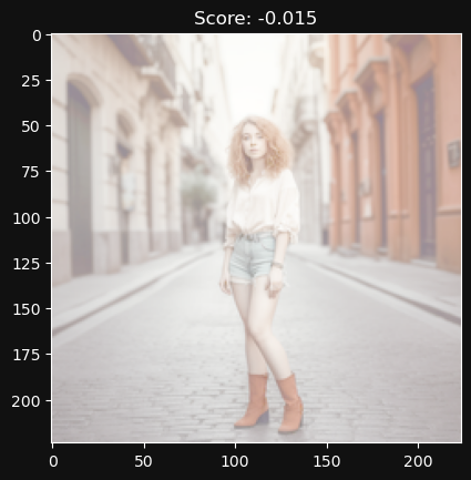
Overexposing a photo seems to decrease the score
Poorly cropping an image seems to decrease the score
Heavily compressing an image didn’t seem to affect the score much
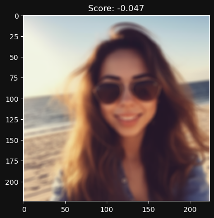
Significantly blurring the image seems to decrease the score
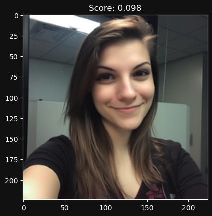
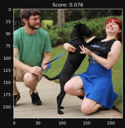
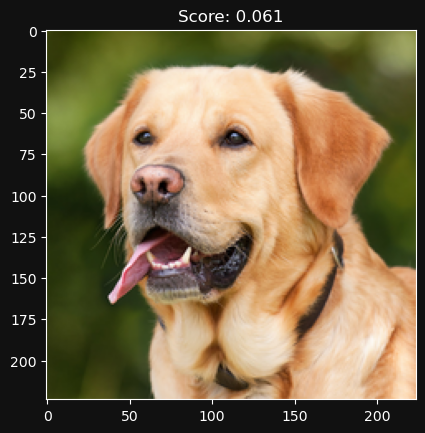
Let’s try a random assortment of photos now and sort them by score (by the way, did you notice all the photos above are AI generated by MidJourney v5?)
Next steps
Use a CLIP model: Based on some preliminary testing, adding CLIP to the current architecture improves accuracy by almost 2 percentage point. Therefore this is a very easy and big win.
Simultaneous train on slight and heavy augmentation transforms: The current largest issue is overfitting. Using data augmentation with too strong transforms is a bit moot because many features that will make a photo good are lost. However, changing the architecture to have 2 heads, one with a smaller (less prone to overfitting) model that trains on a slightly transformed image, and another with a larger (more prone to overfitting) that trains on a strongly transformed image might improve performance.
Conclusion
We have built an AI model that can approximately evaluate the quality of a photo, particularly in terms of social media impact. The code and weights are available on my GitHub.
